Summary: I labeled ~41k query–paragraph pairs on a 5-level relevance scale using Claude Sonnet 4.6 and fine-tuned six cross-encoders with ordinal regression (CORAL). Legal-domain pretraining and model size matter most. legal-swiss-roberta-large reaches a Spearman $\rho$ of ~0.8 against the LLM labels, far ahead of general-purpose models. Article citations in the query are a meaningful signal. Adding section-title context (margin text from the law) on top adds little. After Platt scaling, predicted inclusion probabilities are well calibrated (ECE $\approx$ 0.02), which gives a principled threshold for retrieval.
The series:
- Part 1: the Swiss legal system and the retrieval pipeline.
- Part 2: a heuristic benchmark built from commentary citations, comparing pretrained embedding models.
- Part 3 (this post): LLM relevance labels and a cross-encoder reranker fine-tuned with ordinal regression.
- Part 4: distilling the reranker into the first-stage retriever.
Introduction & Motivation
In Part 2, the heuristic benchmark pointed to the limitations of a single-stage retrieval architecture. With pretrained multilingual embeddings alone, the cited ruling appears in the top 10 for fewer than half of all queries. Retrieving ~100 candidates raises this above 70%, but most of those extra candidates are presumably noise. The “presumably” is important here, since Part 2 also showed the limitations of the heuristic benchmark. It cannot capture the semantic signal and is not reliable enough to serve as a training signal.
This part addresses both issues:
- Reranking with cross-encoders, which read the query and document jointly and can therefore judge relevance with far more context than bi-encoders.
- Replacing the heuristic with LLM judgments, yielding ~41k query–paragraph pairs scored on a 5-level relevance scale by Claude Sonnet 4.6.
Preliminary Testing
Hybrid Retrieval
In addition to the reranking step, some preliminary testing showed that adding a sparse retrieval signal like BM25 marginally helps on the Heuristic Benchmark from Part 2. These traditional retrieval methods use frequency counts of terms in the query and document as well as information about the ubiquity of terms to judge the relevance. As such, rare terms that only appear in few documents have high discriminative power whereas ubiquitous terms are ignored.
sqlite offers FTS5 as a built in keyword search algorithm. In some preliminary testing with trigram indexing I found marginal improvements. Later analyses also showed that paragraphs retrieved by both the sparse and the dense retriever tend to be more relevant.
Since improvements were only marginal, I did not analyze sparse retrieval in more detail at this point. Instead, each method retrieved 30 candidates, which were pooled and reranked by the cross-encoder (see below) keeping the top 30.
Baseline Exploration
I initially benchmarked the following three models on the same heuristic benchmark from Part 2. Retrieval success rates on the benchmark improved on pure dense retrieval for all three models, meaning the cross-encoders were able to successfully increase the rank of relevant documents from the larger retrieved pool of the bi-encoders although only a few percentage points were achieved.
mmarco-multi, a multilingual cross-encoder trained for passage reranking on mMARCO (a machine-translated version of the MS MARCO dataset of Bing queries), outperformed the other two and served as the basis for building the training set. Since this stage only served to choose that model, I don’t report detailed results.
| Alias | Hugging Face Model ID | Base Architecture | Params | Languages | Max Tokens |
|---|---|---|---|---|---|
miniLM-en-de | cross-encoder/msmarco-MiniLM-L6-en-de-v1 | MiniLM (6-layer) | ~22M | English, German | 512 |
mmarco-multi | cross-encoder/mmarco-mMiniLMv2-L12-H384-v1 | mMiniLMv2 (12-layer) | ~117M | Multilingual | 512 |
mxbai-large | mixedbread-ai/mxbai-rerank-large-v1 | DeBERTa-v3-large | 435M | English (Primarily) | 512 |
Why Train the Reranker First?
It might seem counterintuitive to first tune the reranker instead of the retriever. The reason for this order is the architectural difference between cross-encoders and bi-encoders, which strike a trade-off between latency and contextual awareness:
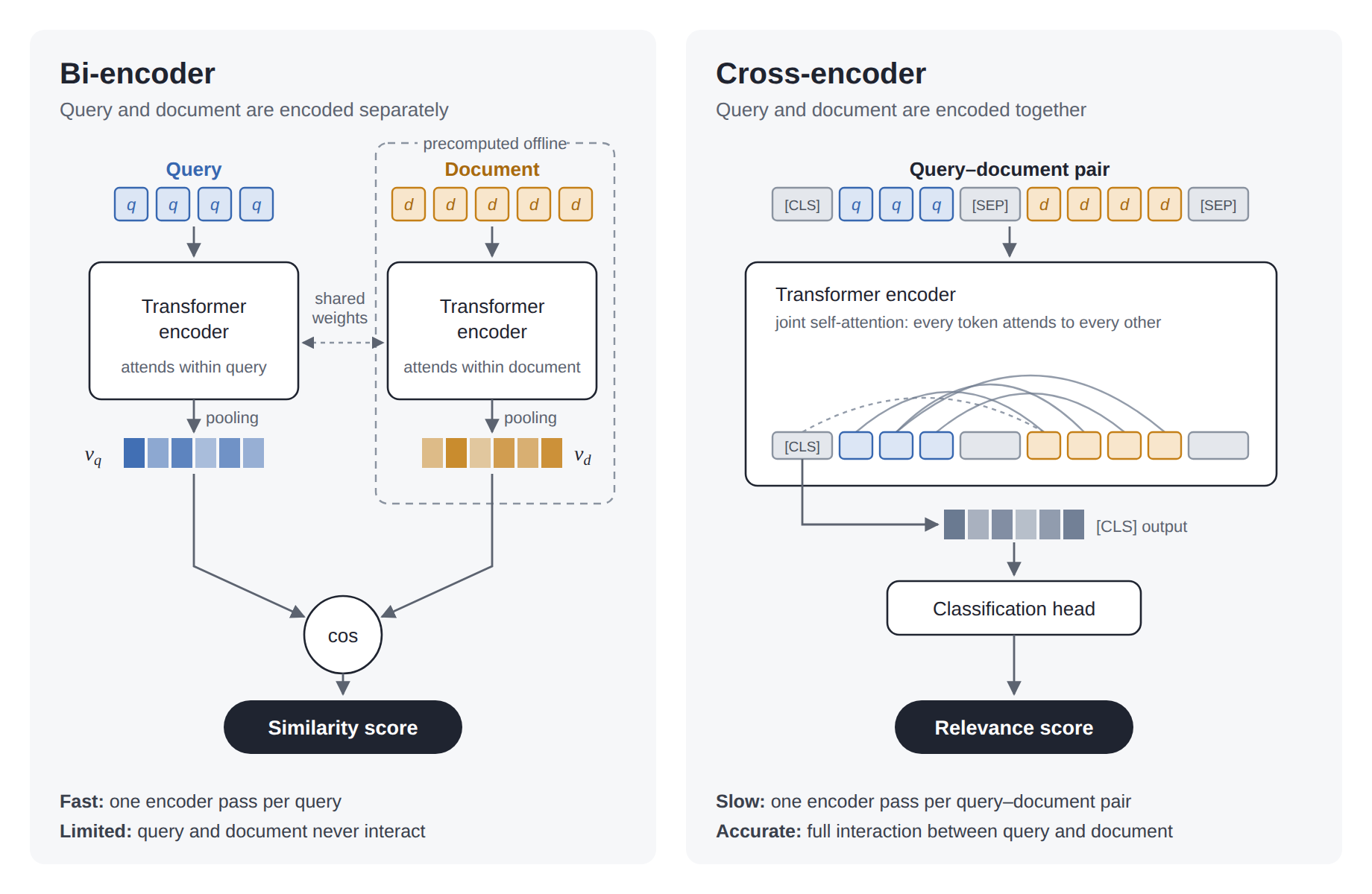
Bi-encoders embed the query and document separately and score relevance by the cosine similarity of the two vectors (a dot product of normalized embeddings). The document embedding is computed once, independent of any query, so all relevance information has to be encoded statically in the embedding space. This makes bi-encoders fast enough to search the full corpus.
Cross-encoders, on the other hand, take the query and document concatenated as a single input and run them through the transformer together. Because self-attention1 operates over the whole sequence, every query token can attend to every document token and vice versa. The model can weigh contextual interactions much more finely, at the cost of a full forward pass for every query–document pair.
Following Hofstätter et al. (2020)2 on cross-architecture knowledge distillation, the plan was to first teach the more expressive cross-encoder the relevance signal from Claude’s judgments, and then use it as a cheap teacher for fine-tuning the bi-encoder, without further API calls. The knowledge distillation step will be discussed in Part 4 of this series.
What is Attention? The setup of attention1 is very elegant. Each token is projected into three vectors: a Query ($\mathbf{q}$), a Key ($\mathbf{k}$) and a Value ($\mathbf{v}$). The relevance of query-token $i$ for key-token $j$ is the dot product $\mathbf{q}_i\cdot \mathbf{k}_j$, scaled by $1/\sqrt{d_k}$ and passed through a softmax to produce attention weights. The output for each token is then a weighted sum of all value vectors, so every token can attend to every other token. In a cross-encoder, query and passage share one sequence, so their tokens interact directly in every layer. A bi-encoder never lets them interact at all (see the illustration below).
Training Data
Extracting Relevance Signal
In order to teach the cross-encoder a more fine-grained and useful signal than a simple binary “relevant” vs. “non-relevant”, I designed the following 5-level ordinal scale (0-4):
| Ordinal Scale | Label | Description | Example Query: “Prescription period and notification duty of the buyer for defective goods (Art. 201, 210 OR)” |
|---|---|---|---|
| 0 | Non-Relevant | An entirely different area of law or a clearly different legal question without a connection to the query | Prescription period for a criminal offence (entirely different area of law) |
| 1 | Thematically Relevant | Same area of law but a clearly different legal question such that a lawyer would acknowledge it but not use it as a reference | Prescription period for defective work in a work-contract (“Werkvertrag”, OR 363) |
| 2 | Partially Relevant | Partial aspect or a related legal notion, which is helpful but not central (e.g., a discussion of general principles without a connection to the specific issue) | General principles of warranty in sales contracts without treating prescription period or notification duties |
| 3 | Relevant | Core legal question substantially covered but missing some aspect of the query | Only the prescription period but not the notification period is treated |
| 4 | Directly Relevant | Query treated in all substantial aspects such that a lawyer would cite it as a primary source | Both aspects are treated. |
To calibrate the LLM-judge, the system prompt included an example for each category, similar to the ones given in the above table. More details on the model selection can be found below.
Ordinal Scale vs. Ranking
Note that the LLM was instructed to judge relevance on an ordinal scale instead of rank a set of passages. While the latter is found prominently in the LLM-as-a-judge literature, in the RAG context, the cross-encoder should not only learn to rank but also predict relevance to avoid bloating the LLMs context with irrelevant information. Therefore, ranking and top-k retrieval are not well-suited. Instead, as discussed in the training section, the model is trained to predict whether the document passes each of four relevance thresholds.
Training Set Creation
The dataset was constructed by selecting the top 30 candidates as predicted by the untrained mmarco-multi from a pool of 60 candidates comprising 30 candidates retrieved by snowflake-arctic (dense retrieval) and 30 candidates retrieved by keyword search using FTS5 in sqlite (analogous to BM25). In cases where no exact match (i.e., a match on the intended ruling id and consideration number) was obtained, the corresponding “ground-truth” consideration was subsequently added to the candidate set to ensure that the cross-encoder always has positive examples.
A preliminary run in which Claude judged candidate pools built this way showed that all five relevance levels were fairly well represented, which validates the construction. The pools also contain many hard negatives, i.e., paragraphs that the retrievers ranked highly but Claude judged as non-relevant. Alongside strong positives, these are the most informative examples, especially where the model is confidently wrong.
From ~1'400 queries I obtained ~41k labeled pairs, distributed as follows. The data is clearly skewed toward the lower levels with only ~14% of pairs labeled Relevant or better.
Directly Relevant | Relevant | Partially Relevant | Thematically Relevant | Non-Relevant |
|---|---|---|---|---|
| 5.3% | 8.9% | 25.0% | 42.7% | 18.1% |
Judge Model Selection
I compared Claude Sonnet 4.6, Gemini 3 Flash, Gemini 3.1 Pro on a small set of samples and manually inspected the results. Gemini 3 Flash had a tendency to inflate relevance scores whereas Gemini 3.1 Pro was the harshest critic. Notably, it paid most attention to missing aspects of the query, relating to the distinction between 3 and 4. Claude Sonnet 4.6 tended to side with Gemini 3.1 Pro and calibration using an example made Sonnet also pay greater attention to missing aspects.
Gemini required medium to high thinking budgets for good results, which consumed a significant number of reasoning tokens. On small samples of 200 pairs, Gemini 3.1 Pro and Claude Sonnet 4.6 consistently agreed exactly on 80–90% of labels and within ±1 on all of them. Given comparable quality, I chose Claude Sonnet 4.6 for cost reasons.
Label Consistency Analysis
After some initial training runs, it became clear that the most difficult separation to learn was between 2 (Partially Relevant) and 3 (Relevant), which makes sense intuitively. To assess the strength of the signal, I ran a 200-pair rescore experiment on a stratified random sample of 100 pairs initially rated at 2 and 100 pairs rated at 3 by Claude.
The rationale of this experiment was that if Claude reproduces its own labels consistently, the 2/3 boundary is at least well defined from the judge’s perspective, and the cross-encoder has something stable to learn. If the labels flipped frequently, the fine-grained scale would add noise rather than signal.
The rescoring experiment showed 82.5% exact and 99.5% soft (±1) agreement. Only ~7% of pairs swapped between 2 and 3, the remaining disagreements mostly moved outward (2 to 1 or 3 to 4). The boundary is therefore stable enough to learn, which supports using the 5-level scale. To avoid miscalibration I sampled a small batch of pairs and found that relevance judgments were well-reasoned throughout.
Setting
mmarco-multi served as the baseline. All models were trained on the ~41k query–passage pairs with an approximately 80/20 split. To prevent data leakage, the split was made at the article level rather than the pair level, so the validation set only contained queries on articles the model had never seen. The realized split was therefore ~31.5k training and ~10k validation pairs. I used a learning rate of 1e-5 and a batch size of 16 throughout and did not perform further hyperparameter tuning. The model was evaluated on the validation set at regular intervals, and the checkpoint with the best overall Spearman $\rho$ rank correlation was kept.
Spearman’s rank correlation $\rho$ measures the monotonic relationship between predicted and true orderings. A $\rho$ of $1.0$ means perfect agreement in rank order while $0$ means no relationship.
Note that Spearman’s $\rho$ only compares orderings, which suits ordinal labels whose levels are not evenly spaced. I report it both pooled over all validation pairs and per query. The per-query value measures reranking quality proper whereas the pooled value additionally rewards scores that are comparable across queries, which matters for a single global inclusion threshold. Because every CORAL threshold probability is a strictly increasing function of one shared logit, $\mathbb{E}[Y]$ and $P[Y \geq 3]$ order the pairs identically. Ranking and inclusion decisions therefore rest on a single score.
Spearman’s $\rho$, however, rewards getting that order right across all five levels, not specifically at the boundary between levels 2 and 3. I therefore complement it with AUPRC for $Y \geq 3$ and with the ECE after Platt scaling in later sections. In hindsight, AUPRC(Y≥3) would have been a better metric for checkpoint selection. The model rankings were the same under both.
Ordinal Regression (CORAL)
The issue with standard regression when applied to an ordinal scale like the one presented here is that it assumes the distance between the labels to be uniform. In reality, the step from Non-Relevant (0) to Thematically Relevant (1) may be very different to the step from Partially Relevant (2) to Relevant (3).
Furthermore, for a RAG pipeline, a good ranking order isn’t enough. Instead, we want a principled and interpretable inclusion threshold to decide exactly which passages make it into the LLM’s context window.
CORAL (Rank Consistent Ordinal Regression) proposed by Cao et al. (2020)3 provides this. It breaks ordinal regression down into K−1 cumulative binary tasks, i.e., predicting for each hurdle if a given document passes it. Architecturally, one can take the single logit from the pretrained model and add 4 learnable bias offsets to the model.
Formal Definition
Formally, let $z\in \R$ be the final pre-activation output of the cross-encoder and let $b_i \in \R, \quad i\in \{1,2, 3, 4 \}$ be the bias weights. The probability of surpassing the relevance threshold for level $i$ is then given by: $$P[Y\geq i] = \sigma(z+b_i), $$ where $\sigma: \R \to (0, 1)$ is a sigmoid activation, outputting a valid probability.
This gives us cumulative probabilities for each threshold. Finally, we can rank the relevance of a batch of documents by their expected relevance defined by: $$\mathbb{E}[Y]=\sum_{k=1}^{K-1}k\cdot P[Y=k] = \sum_{k=1}^{K-1}P(Y≥k),$$ where $K$ is the number of classes ($5$ here) and the second equality follows by regrouping: $$\sum_{k=1}^{K-1}P(Y≥k) = \sum_{k=1}^{K-1}\left(\sum_{i=k}^{K-1} P[Y=i]\right) = \sum_{i=1}^{K-1}i\cdot P[Y=i],$$
Notice that each probability $P[Y=i]$ appears in exactly $i$ of the inner sums (once for every $k \le i$), which yields the factor $i$.
Monotonicity Guarantee
The elegance of CORAL is that it maintains the monotonicity of the ordinal scale in its predictions, meaning it avoids inconsistent predictions where the model for instance predicts $P[Y\geq 3] = 0.52$ but $P[Y\geq 2] = 0.24$.
Intuitively, given a single shared logit, the only way to minimize the cumulative binary cross-entropy across all thresholds simultaneously is to place the biases in decreasing order ($b_1>b_2>b_3>b_4$), so that the easiest threshold ($Y\geq 1$) has the highest offset. Cao et al. (2020)3 formally prove that rank consistency holds at any global optimum of the loss.
Platt Scaling: Calibrating the Model’s Confidence
While we have a theoretical guarantee that the output of our model is a valid probability, there is no guarantee that this probability aligns with the empirically observable probabilities. Suppose we took a batch of samples for which the model said $P[Y\geq 3] = 0.8$ and we found that only half the samples instead of $80$% were relevant. Then there would be a clear disconnect between the model’s confidence and its empirical accuracy.
Interestingly, while modern neural networks are achieving increasingly accurate predictions, research suggests that they are also often overconfident and miscalibrated.4
Measuring the Calibration of a Model
Following Guo et al. (2017)4, a model is said to be perfectly calibrated if its predicted probabilities match observed frequencies. In our setting, each CORAL threshold is a binary prediction, so for a threshold $k$ with predicted probability $\hat p_k = \hat P[Y \geq k]$, perfect calibration means $$P[Y \geq k \mid \hat p_k = p] = p, \quad \forall p\in [0, 1].$$ Of all pairs for which the model predicts $0.6$, exactly 60% should actually reach level $k$.
The Expected Calibration Error (ECE) measures the deviation from this ideal. Predictions $\hat p_k$ are grouped into $M = 10$ equal-width bins $B_1, \dots, B_M$. For each bin, $\bar p_{B_m}$ is the average predicted probability and $\text{freq}_{B_m}$ is the share of its pairs that actually reach level $k$. The ECE is the absolute gap between the two, averaged over bins and weighted by bin size:
$$ECE_k = \sum_{m=1}^{M} \frac{|B_m|}{n}\bigl|\text{freq}_{B_m} - \bar p_{B_m}\bigr|.$$
The reliability diagram below plots these two quantities against each other to visualize skew. I report $\text{ECE}_3$, i.e., for the inclusion threshold $Y \geq 3$.
Calibrating a Trained Model
Now that we are able to determine any miscalibration, we should also think about how to remediate it:
- Platt Scaling (Platt, 1999)5 fits a logistic regression on the model’s raw output to learn a calibration mapping. For each cumulative threshold $k$, we fit parameters $a_k, b_k$ such that the calibrated probability is: $$P_{\text{cal}}(Y \geq k) = \sigma(a_k \cdot \text{logit}_k + b_k),$$ where $\text{logit}_k = \log\frac{P(Y \geq k)}{1 - P(Y \geq k)}$ is the log-odds of the model’s raw prediction. The parameters are fitted on a held-out calibration set by minimizing the negative log-likelihood. In the cross-validation setup, Platt parameters are fitted on the pooled out-of-fold predictions, ensuring that every data point is calibrated by a model that never trained on it.
- Temperature Scaling (Guo et al., 2017) is a simpler alternative that uses a single scalar $T > 0$ to soften or sharpen all logits: $\text{logit}_{\text{cal}} = \text{logit} / T$. While reducing calibration to a single parameter, it applies the same correction uniformly across all confidence levels and thresholds, which is likely too restrictive for our setting where different thresholds may be miscalibrated in different directions. I therefore focused on the per-threshold Platt approach first.
Query Expansion
Around 90% of queries from the dataset contain references to legal provisions. Intuitively, the law is cited to support a statement with authoritative context. As discussed in Part 1, legal articles need to be “general” and “abstract”. They state a legal rule in a general manner without any prose and generally without specific fine-grained subcases. The refinement of formal legal provisions is left to the executive branch to specify at the level of “Verordnungen” and to the courts.
But whereas a lawyer has the rough content of the article in their head when citing or reading Art. 5 BV, a model needs to learn what the reference means. To facilitate this, I experimented with query expansion, whereby I parse the article reference and add it at the end of the query separated by a newly added <ART> special-token, which guarantees that the tokenizer parses it as one piece and assigns it a newly initialized embedding. The intention behind this is to help the model learn the structural distinction between the query-parts.
Expansion Strategy
I experimented with two expansion strategies:
- Including the entire article and section titles to provide the structural and specific context.
- Including only the section titles to provide the structural context.
The first version was used for the Longformer architecture, the second was used for the RoBERTa models due to the limited context window. An ablation on the expansion for the RoBERTa models is presented at the end, where I compare how references and expansion affect retrieval quality.
Here is a sample:
Original Query:
---------------
Schutzpflicht des Staates gegenüber Versammlungen bei drohenden
Gegendemonstrationen gemäss Art. 22 BV und polizeirechtliches Störerprinzip
                                        ↓

Expanded Query, Version 1: Include Section Titles and Article
---------------------------------------------
Schutzpflicht des Staates gegenüber Versammlungen bei drohenden
Gegendemonstrationen gemäss Art. 22 BV und polizeirechtliches Störerprinzip
<ART> [Art. 22 BV]:
2. Titel: Grundrechte, Bürgerrechte und Sozialziele > 1. Kapitel: Grundrechte > Versammlungsfreiheit
1 Die Versammlungsfreiheit ist gewährleistet.
2 Jede Person hat das Recht, Versammlungen zu organisieren, an Versammlungen teilzunehmen oder Versammlungen fernzubleiben.

Expanded Query, Version 2: Only use the Section Titles
--------------------------------------
Schutzpflicht des Staates gegenüber Versammlungen bei drohenden
Gegendemonstrationen gemäss Art. 22 BV und polizeirechtliches Störerprinzip
<ART> [Art. 22 BV]:
BV > Grundrechte, Bürgerrechte und Sozialziele > Grundrechte > Versammlungsfreiheit
Results
I fine-tuned and compared the models listed in the table under this set-up. Particularly noteworthy are the pretrained models by Niklaus et al. (2024)6. The authors finetuned two pretrained model architectures and tokenizers on their MultiLegalPile dataset, which comprises roughly 700GB of legal text from various jurisdictions:
- XLM RoBERTa (base / large) (Conneau et al., 2019)7, which is a multilingual version of RoBERTa8, trained on 2.5TB of data spanning 100 languages.
- Longformer (base, no large available) (Beltagy et al., 2020)9, which is designed to extend the attention window of the transformer layers efficiently by using a sliding window approach.
Note, if we let all tokens interact with each other in full attention, we obtain quadratic complexity, which works for smaller windows like RoBERTa’s (512 token limit) but does not readily scale to many thousands. The Longformer slides a 512 token window across the document, which lets the query tokens interact with much longer documents while scaling linearly. This is interesting for long documents and query expansion approaches, where additional context is added to the query (see below).
I benchmarked both architectures and compared RoBERTa models pretrained on the entire MultiLegalPile with models pretrained purely on Swiss legal sources. For details on pretraining, see Niklaus et al. (2024)6.
The following table gives an overview of the benchmarked models and their aliases used in the subsequent analysis.
| Alias | Hugging Face Model ID | Base Architecture | Params | Max Tokens | Short Description |
|---|---|---|---|---|---|
mmarco-multi | cross-encoder/mmarco-mMiniLMv2-L12-H384-v1 | mMiniLMv2 (12-layer) | ~117M | 512 | Baseline multilingual compact cross-encoder pre-trained on MS-MARCO Bing searches. |
roberta-base | FacebookAI/xlm-roberta-base | XLM-RoBERTa (Base) | ~278M | 512 | Baseline multilingual model pretrained on general web text (CommonCrawl). |
legal-base | joelniklaus/legal-swiss-roberta-base | XLM-RoBERTa (Base) | ~278M | 512 | Domain-adapted model pretrained on Swiss MultiLegalPile corpus. |
legal-multi-large | joelniklaus/legal-xlm-roberta-large | XLM-RoBERTa (Large) | ~550M | 512 | High-capacity multilingual legal model pretrained on the full MultiLegalPile corpus. |
legal-large | joelniklaus/legal-swiss-roberta-large | XLM-RoBERTa (Large) | ~550M | 512 | High-capacity domain-adapted model pretrained on Swiss MultiLegalPile corpus. |
legal-long | joelniklaus/legal-swiss-longformer-base | Longformer (XLM-R Base) | ~278M | 4096 | Domain-adapted model utilizing windowed attention for extended legal context pretrained on Swiss MultiLegalPile corpus. |
Analogously to the benchmarks in Part 2, we now want to compare the models on different dimensions and assess areas for improvement:
- Correlation to assess if the models’ relevance predictions are in line with the dataset.
- Score distributions and class separation to assess the discriminative power and certainty of a model.
- Precision-Recall to assess the trade-off between finding relevant documents but not retrieving too many false positives.
- Calibration to assess and calibrate the uncertainty of the models’ outputs.
Training / Validation Methodology
Unless specifically marked as cross-validation results, all of the following results were obtained from a single training run on 5 epochs with an ~80/20 train-validation split, choosing the best model as measured on the overall Spearman correlation on the validation set at regular intervals. The training and validation set are strictly split by articles such that the model never sees a query for an article it was trained on in testing.
Where results are marked as cross-validated, they are based on a 5-fold cross-validation with the same approach as above. Cross-validation improves the robustness of the results since every data point is included in the result exactly once, when included in the out-of-fold set. The CV results include all out-of-fold predictions. Cross-validation was only performed for a selection of models due to compute limitations. Across all categories, cross validation confirms the consistency of the performance such that the single training run results can be deemed representative.
During k-fold cross-validation we split the dataset into k sets and train k models, each on a different subset of $k-1$ folds, and evaluate on the $k$-th fold. Averaging over all folds gives us a more robust estimate of the true generalization error since we use every data point in training and in evaluation but never validate on training data to avoid leakage.
Summary
To give an overview of the results presented below, three clear trends emerge, with one surprise:
Strong Learning: The models learn the relevance signal well as indicated by the Spearman correlation overall and per Query, which measures the relative alignment of the model’s prediction with the true labels (Claude’s judgment).
Capacity matters: For RoBERTa, the
largemodel performs significantly better across all metrics than thebasemodel, indicating that model capacity helps with learning the signal. The only case, where this relation is flipped is betweenmmarco-multiandroberta-base. Even thoughroberta-baseis a significantly larger model, it falls behindmmarco-multiquite significantly. This may be explained by the next factor.Pre-Training matters
Domain-specific language: The models pre-trained by Niklaus et al. (2024)6 on legal sources adapted to the new domain significantly better than the base model. Notably, the
swissversion, trained on Swiss documents, outperformed themultiversion, which was trained on the entire MultiLegalPile6.Training Distribution: The superior performance of the small
mmarco-multimodel over the largerroberta-base, both of which were only pre-trained on general, multi-language text, is likely due to the structure of the training sets. In particular,mmarco-multiwas trained as a reranker on the MS MARCO dataset of Bing searches10, which naturally entails the query-document structure and relevance signal.roberta-base, on the other hand, was trained by masked language modeling.7
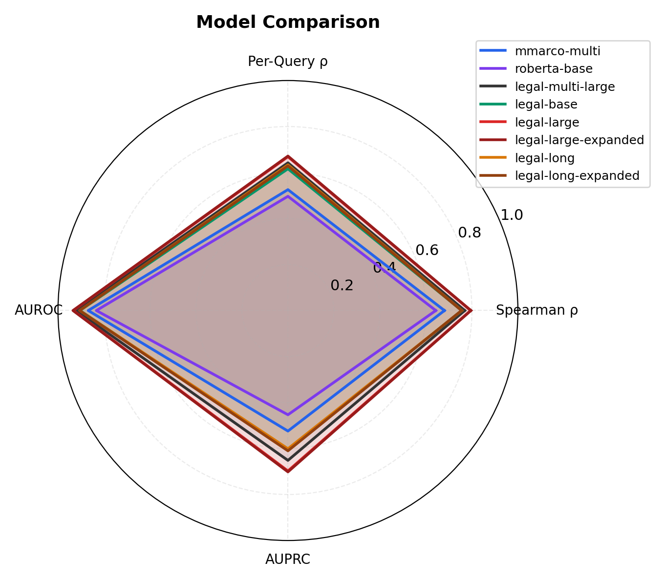
legal-large and legal-large-expanded lead on every metric by a significant margin. Between the two, the differences are within noise for a single run (e.g., overall $\rho$ 0.7958 vs. 0.7945), so they can be considered tied. No large Longformer was available but at the base size, the Longformer performs on par with legal-base.
Overview
| Model | Spearman (overall) | Spearman (per-query mean) | Spearman (per-query median) | % negative Spearman | AUROC ($\geq 3$) | AUPRC ($\ge 3$) |
|---|---|---|---|---|---|---|
mmarco-multi | 0.6806 | 0.5256 | 0.5635 | 2.8% | 0.8688 | 0.5242 |
roberta-base | 0.6430 | 0.4967 | 0.5276 | 2.3% | 0.8333 | 0.4533 |
legal-base | 0.7556 | 0.6162 | 0.6433 | 1.4% | 0.9043 | 0.6071 |
legal-multi-large | 0.7690 | 0.6423 | 0.6826 | 0.0% | 0.9217 | 0.6517 |
legal-large | 0.7945 | 0.6687 | 0.7042 | 0.0% | 0.9337 | 0.6976 |
legal-large-expanded | 0.7958 | 0.6716 | 0.7072 | 0.3% | 0.9348 | 0.7017 |
legal-long | 0.7561 | 0.6331 | 0.6612 | 0.6% | 0.9057 | 0.6011 |
legal-long-expanded | 0.7549 | 0.6288 | 0.6597 | 0.6% | 0.9063 | 0.6100 |
Score Distributions by Relevance
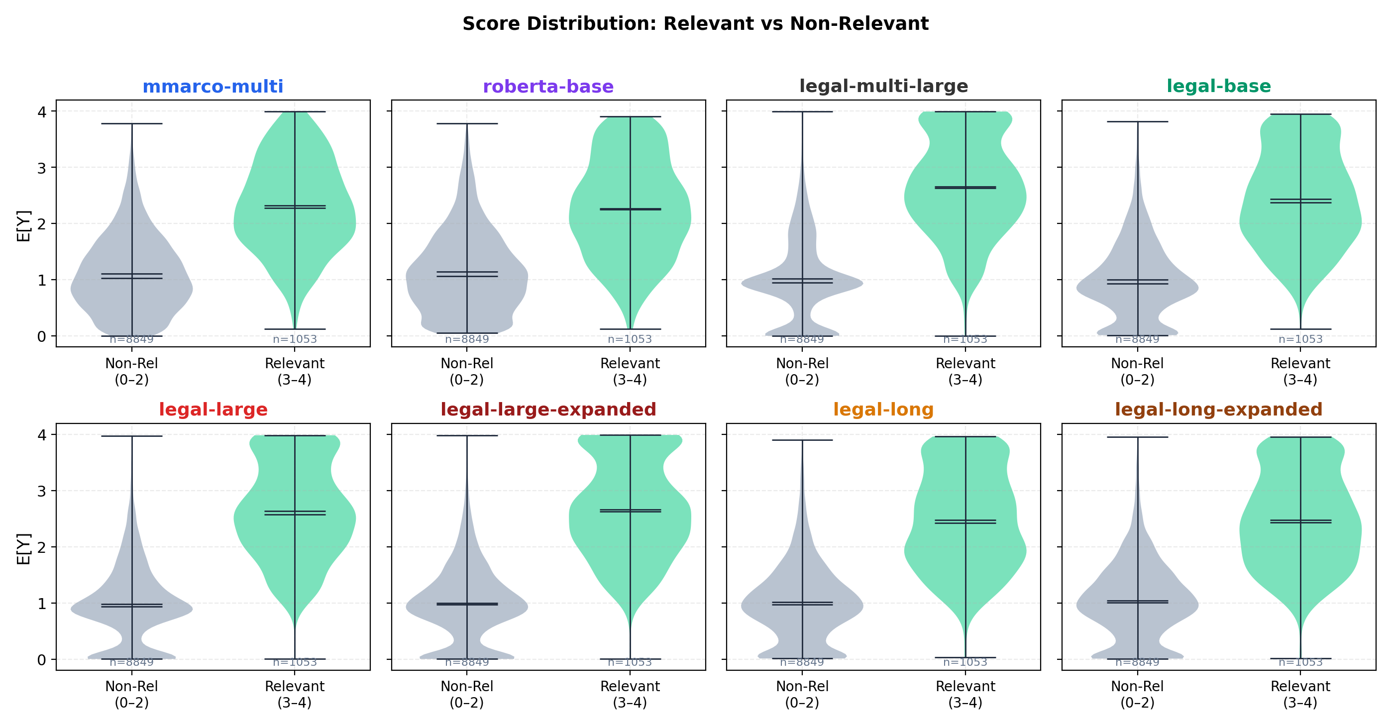
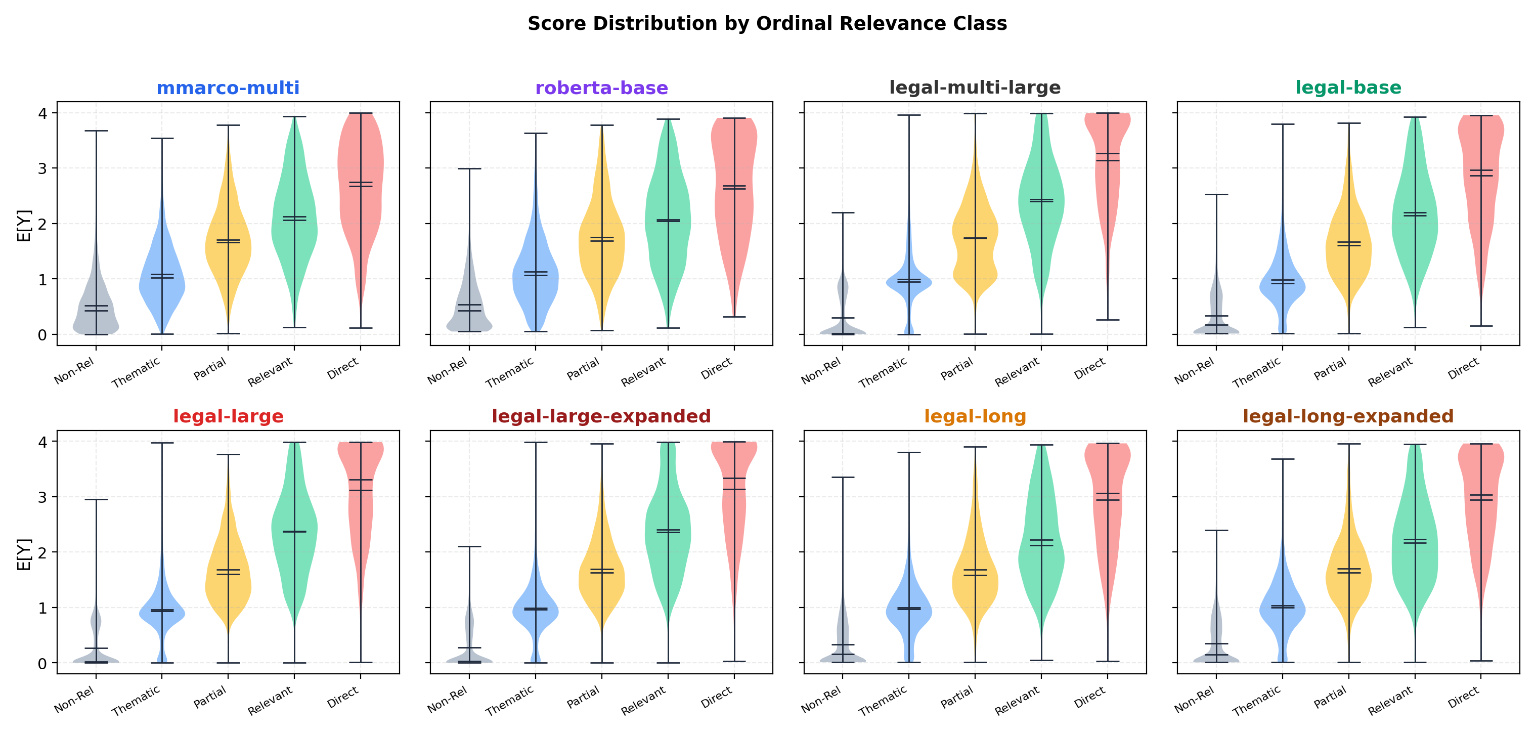
To judge how well a model learned to predict the relevance of a document for a given query, we can consider the expected value assigned to a document by the model. In particular, the better a model learns to predict the relevance, the more confident its predictions should be and yield a clear separation of the classes. To visualize this, the plots below show the distribution of the predicted relevance within:
- the binary class of non-relevant (labels 0-2) and relevant (labels 3&4)
- within each class of label.
A perfect model would produce only a point for each label (each prediction coincides with the true label). A confident model should show a clear separation of the classes. The better the separation, the more signal the model has learned to use for its judgment. Some overlap is to be expected given the difficulty of the task, even for a human-expert.
Results
Looking at the plots below, these patterns are indeed confirmed by the data. Whereas general-purpose models mmarco-multi and roberta-base show large overlaps in the expected values between the classes, legal-large and legal-large-expanded, the best-performing models, show a much clearer separation.
Class Separation
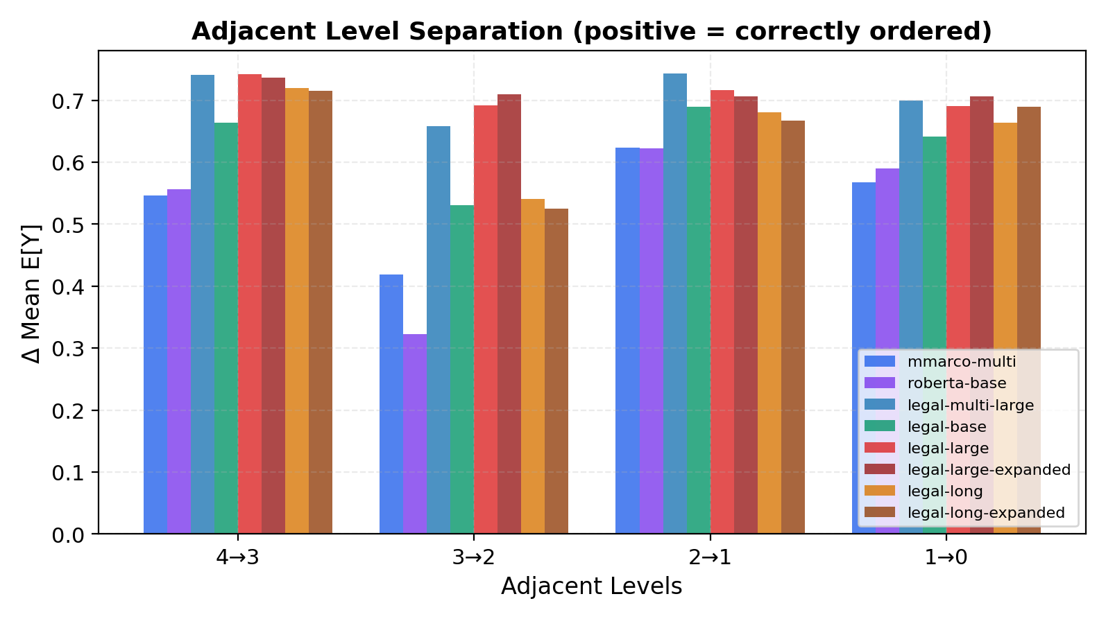
We can also measure the separation of classes by considering the difference in the mean expected value $\mathbb{E}[Y]$ for each class of labels. The separation between 3$\to$2 is particularly important, since it decides on the inclusion of a document in the search. Again, legal-large and legal-large-expanded achieve the largest separation by a wide margin, notably also much wider than at the other junctions.
Confusion Matrix
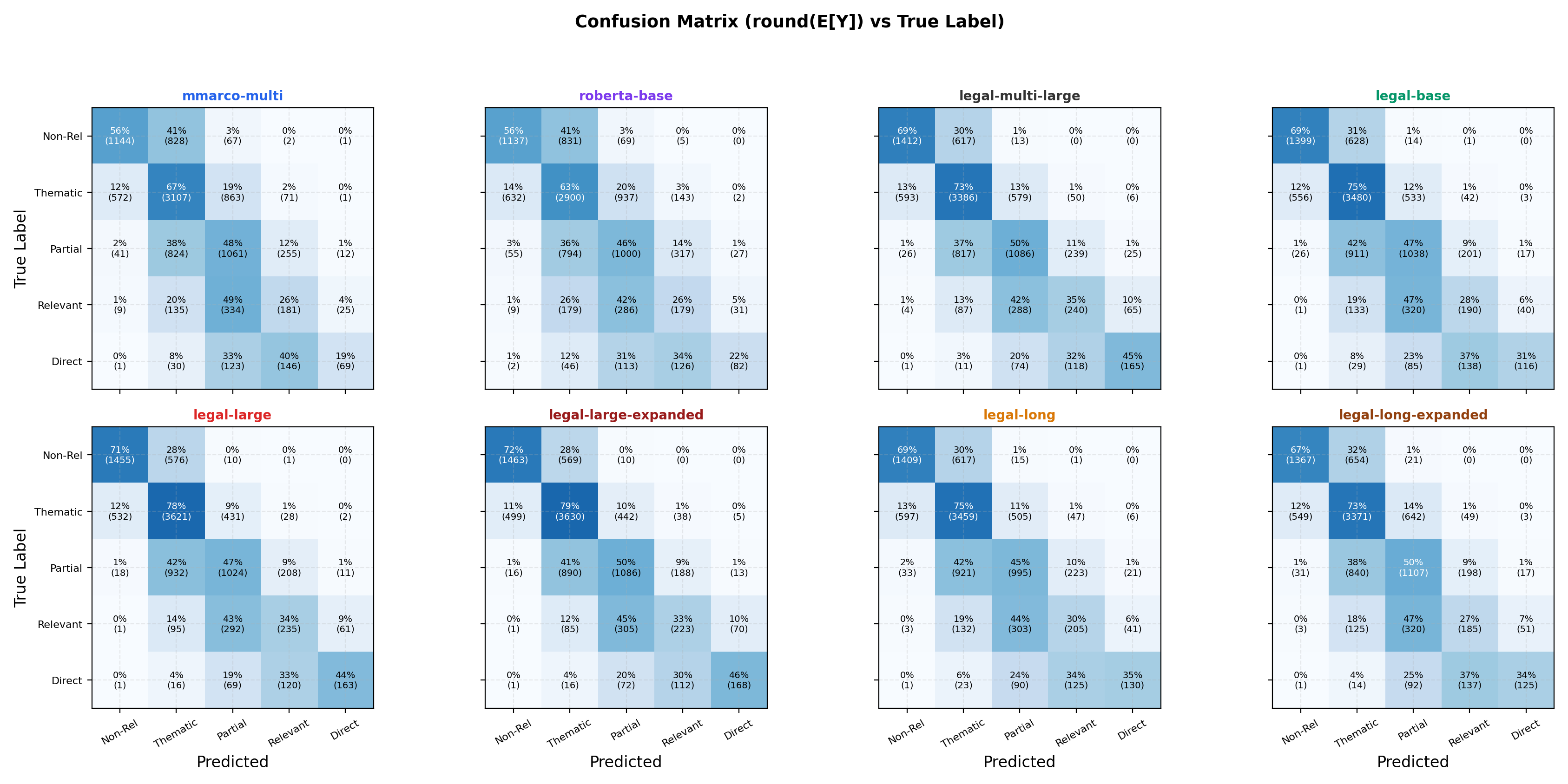
Finally, we can consider the confusion matrix to assess:
- How many documents are misclassified
- In which direction the models tend to misclassify, i.e., if they over- or underrate a document’s relevance.
Looking at the results, we find two trends
- Misclassification increases with relevance indicated by the fading blue on the diagonal. But whereas the fade continues for the weaker models (
mmarco-multiandroberta-base), there is a significant jump in accuracy forlegal-largeandlegal-large-expandedfrom label 3 (33% accurate) to label 4 (46% accurate). Still, they misclassify a large share of documents and for label 3, the dominant predicted class is label 2. This makes sense given the vagueness of the border between partially relevant and relevant (see the definitions above). - Misclassification is strongly biased to underrate a document’s relevance. This is likely also attributable to the overrepresentation of label 0 and 1 documents in the training set, such that the “safe guess” to minimize the loss is to underestimate the relevance.
Query Expansion Ablation
To evaluate the effect of article citations and expansion with section titles on the cross-encoder’s ranking quality, I ran a small ablation experiment. Specifically, I extracted 181 queries, yielding ~5,100 query–passage pairs from the 5-fold CV hold-out sets where the query contains:
- one or multiple citations, all strictly in brackets (e.g., “Gewährleistung im Kaufvertrag (Art. 184 OR) vs. Auftrag (Art. 394 OR)”).
- a single legal citation only at the end of a sentence (“Gewährleistung im Kaufvertrag gemäss Art. 184 OR”)
In these cases, removing the article citations should maintain a structurally sound sentence. Each pair was then scored by the fold model that never trained on it to isolate the effect of a citation on an unseen sentence.
Four query variants are compared, holding passage and label fixed:
| Condition | Query form | Example |
|---|---|---|
| No Ref | Citation stripped | Rechtsfolgen nichtiger GmbH-Beschluss: Feststellungsklage vs. Anfechtungsklage, Beachtung von Amtes wegen |
| As-Is | Original citation | …Beachtung von Amtes wegen nach Art. 808c OR |
| No Ref + Exp | Stripped + breadcrumb | …Beachtung von Amtes wegen <ART> [Art. 808c OR]: OR > Obligationenrecht > … |
| As-Is + Exp | Citation + breadcrumb | …nach Art. 808c OR <ART> [Art. 808c OR]: OR > Obligationenrecht > … |
Ranking quality
| Condition | Mean ρ | Median ρ | Δ vs No Ref |
|---|---|---|---|
| No Ref | 0.598 | 0.636 | - |
| As-Is | 0.659 | 0.691 | +0.060 |
| No Ref + Exp | 0.659 | 0.684 | +0.060 |
| As-Is + Exp | 0.665 | 0.680 | +0.067 |
All four conditions maintain strict monotonicity across all five relevance levels, so the model never “breaks” but just becomes less precise without the citation.
E[Y] by true relevance label
| Label | Scale | No Ref | As-Is | As-Is + Exp |
|---|---|---|---|---|
not relevant | 0 | 0.46 | 0.31 | 0.28 |
thematically related | 1 | 1.14 | 1.08 | 1.07 |
partially relevant | 2 | 1.78 | 1.80 | 1.82 |
relevant | 3 | 2.48 | 2.48 | 2.50 |
directly relevant | 4 | 3.13 | 3.19 | 3.24 |
Key takeaways
The article citation is a meaningful signal (+0.060 $\rho$). The cross-encoder uses it in both directions, assigning relevant passages higher expected values and pushing down non-relevant passages (see
Non-RelevantandThematically Relevant).Expansion adds little on top of the citation: +0.007 $\rho$ from As-Is to As-Is + Exp. However, the section titles can substitute for a missing citation: No Ref + Exp recovers the full +0.060.
Stripping the citation costs ~0.06 $\rho$ without breaking the model. Whether this carries over to queries that never contained a citation is open.
Note that this is a structurally specific subset of 181 out of 1,466 queries, in which the citation sits in brackets or at the end of the sentence after a preposition (German gemäss, nach). A controlled setup, with query generation instructed accordingly, would be needed to validate these findings on semantically richer queries.
Also note that the reported Spearman correlations are computed within each query’s candidate set, aligning with the per-query mean $\rho \approx 0.67$ across the full corpus rather than the overall $\rho \approx 0.8$.
Precision-Recall
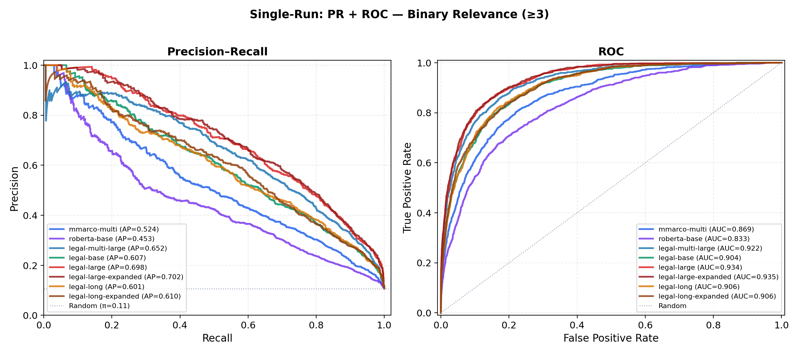
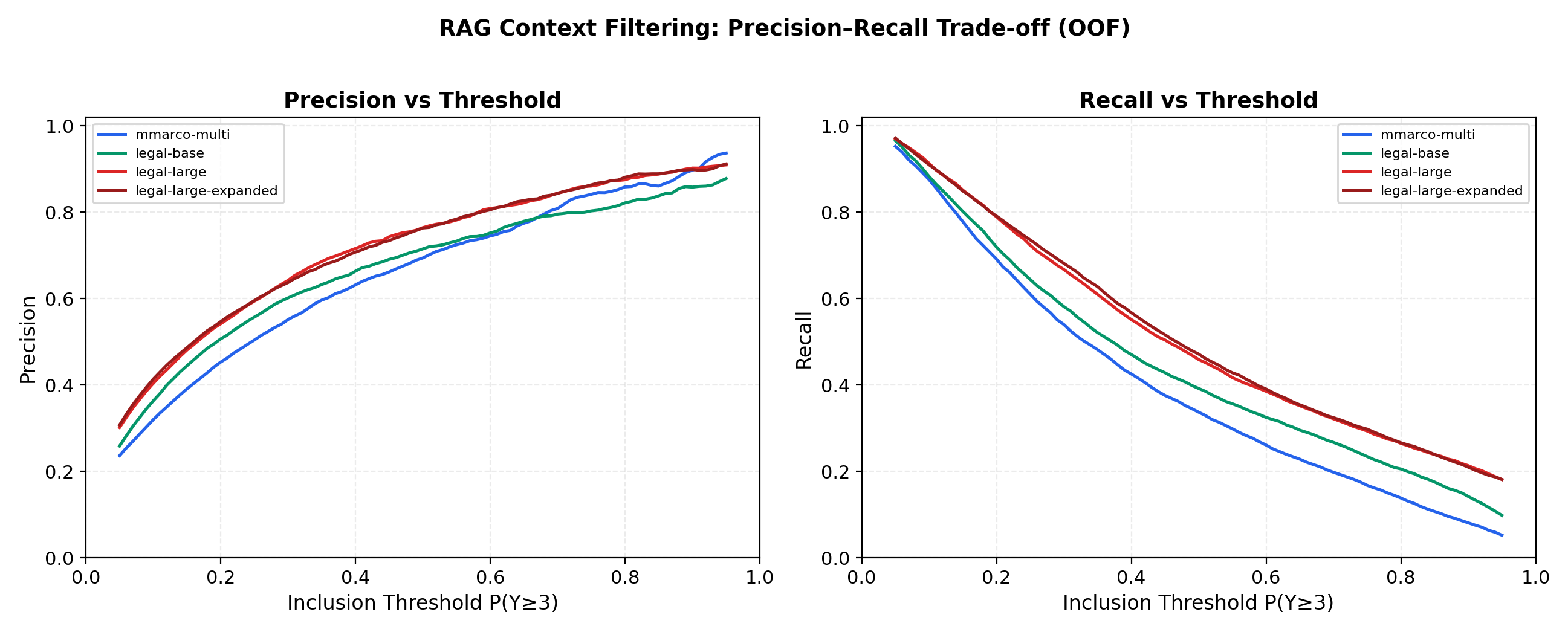
There is an inherent trade-off between Precision and Recall. To retrieve a greater share of the relevant documents and improve Recall, we need to cast a wider net. However, if the added documents from casting a wider net are not relevant, then Precision suffers. By plotting precision vs. Recall and the True Positive Rate vs. the False Positive rate, we can plot the behavior of a model regarding this trade-off. Here, I treat a passage as relevant if its label is at least 3 (Relevant) and include it if the model’s $P[Y \geq 3]$ exceeds a threshold.
Precision is the share of included passages that are relevant: $\frac{TP}{TP+FP}$. A precision of 70% means 7 in 10 passages in the context are relevant.
Recall is the share of all relevant passages that are included: $\frac{TP}{TP+FN}$. A recall of 50% means half of the relevant passages make it into the context.
Both are computed over the pooled candidate pairs of the validation set. Recall is therefore measured relative to the candidates the first stage retrieved, not the whole corpus: a relevant ruling the retrievers never surfaced cannot be counted.
Sweeping the threshold traces out two curves:
- In the precision-recall curve, a better model pushes the curve toward the top-right corner, keeping precision high as recall increases.
- In the ROC curve, a better model pushes the curve further up into the top-left corner, meaning as documents are added to the retrieval pool they are more likely to be True Positives than False Positives.
Again, the ranking of the models is confirmed and legal-large and legal-large-expanded show the best performance:
| Model Alias | Average Precision (AP) | $\Delta$ AP | Area Under ROC (AUC) | $\Delta$ AUC |
|---|---|---|---|---|
mmarco-multi | 0.524 | -0.178 | 0.869 | -0.066 |
roberta-base | 0.453 | -0.249 | 0.833 | -0.102 |
legal-multi-large | 0.652 | -0.050 | 0.922 | -0.013 |
legal-base | 0.607 | -0.095 | 0.904 | -0.031 |
legal-large | 0.698 | -0.004 | 0.934 | -0.001 |
legal-large-expanded | 0.702 | - | 0.935 | - |
legal-long | 0.601 | -0.101 | 0.906 | -0.029 |
legal-long-expanded | 0.610 | -0.092 | 0.906 | -0.029 |
Cross-Validation Results
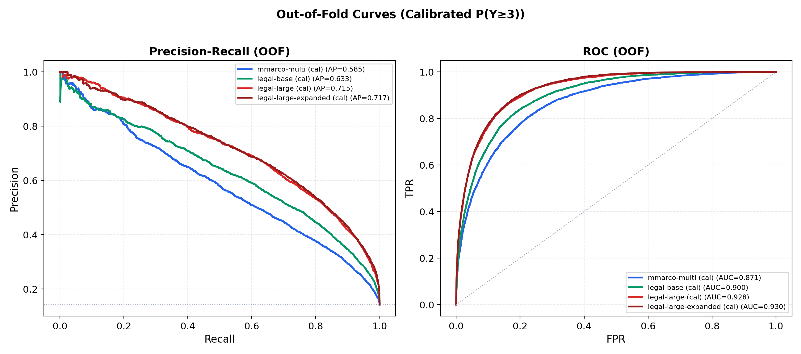
5-fold cross validation confirms these results, which adds a robustness check and suggests that the performance should generalize reasonably well.
RAG Threshold
The precision-recall trade-off directly guides how the final retrieval thresholds for the RAG pipeline need to be set to ensure a sufficiently large but relevant context. In particular, we can make use of the probabilistic nature of the output to obtain a very interpretable trade-off for tuning. As shown in the next section, we can calibrate the model to ensure the probabilities are trustworthy.
The following are the cross-validated results for legal-large-expanded and the curves for all cross-validated models:
- To obtain higher Recall ($0.684$), we would set the threshold at $0.3$, with a Precision of $0.633$, i.e., around 37% of included passages would fall below “Relevant”.
- To obtain higher Precision, we would increase the threshold to $0.5$, yielding a Precision of $0.757$ but reducing Recall to $0.479$.
The right setting depends on how the downstream LLM handles context, which can only be assessed with the full RAG pipeline in place.
| Threshold $P(Y \ge 3)$ | Included Count | Included (%) | Precision | Recall |
|---|---|---|---|---|
| $\geq 0.3$ | 6,376 | 15.4% | 0.633 | 0.684 |
| $\geq 0.4$ | 4,850 | 11.7% | 0.701 | 0.577 |
| $\geq 0.5$ | 3,731 | 9.0% | 0.757 | 0.479 |
| $\geq 0.6$ | 2,960 | 7.1% | 0.797 | 0.400 |
| $\geq 0.7$ | 2,346 | 5.7% | 0.840 | 0.334 |
Calibration
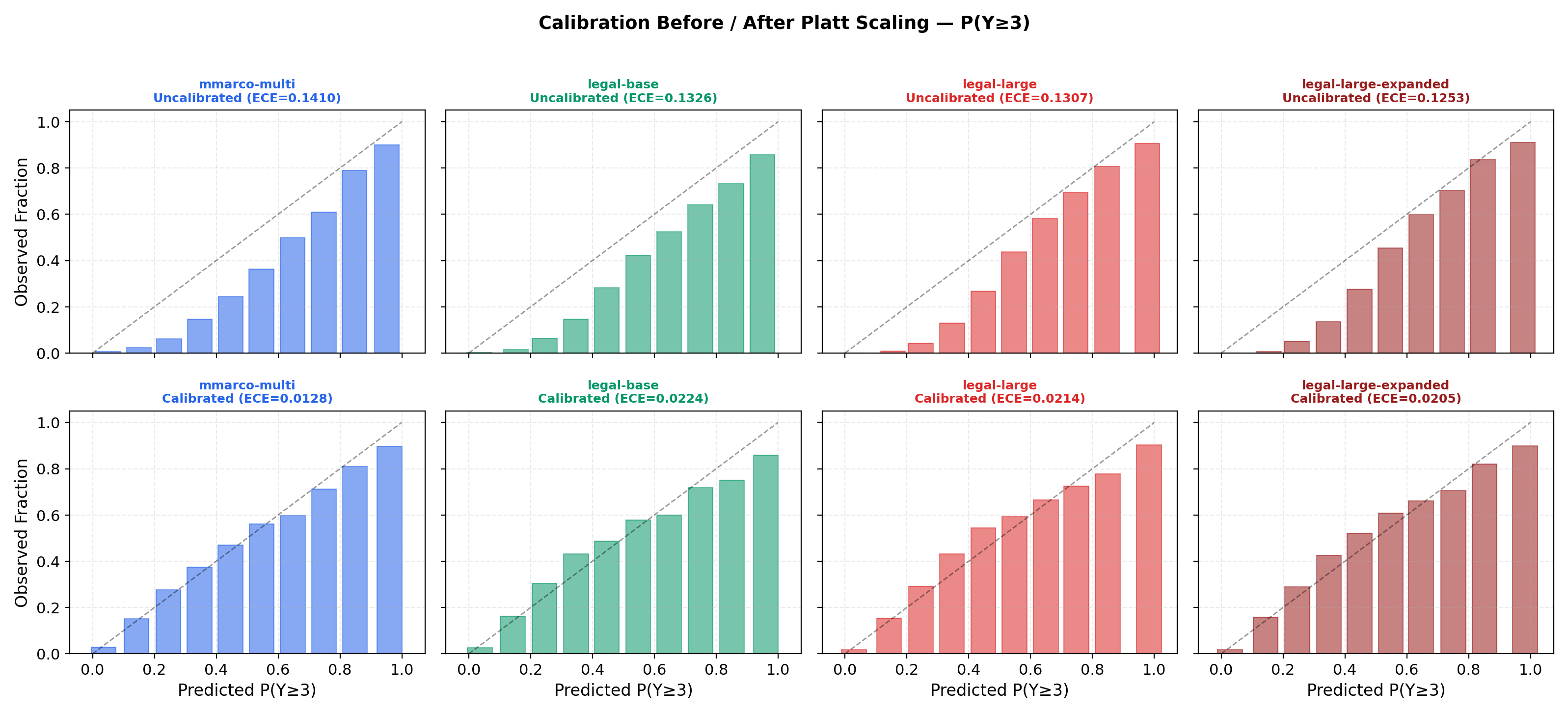
Finally, we consider the calibration of the models, i.e., how well their estimated probabilities reflect the empirical distributions. A perfectly calibrated model would strictly follow the diagonal identity line in the plots below. For the uncalibrated models in the top row, the out-of-fold predictions from cross validation show that the models systematically overestimate the probability for the low-confidence cases but are quite well-calibrated from $P=0.5$ on.
Platt scaling yields strong improvements. For the inclusion threshold $Y \ge 3$, cross-fitted calibration reduces the ECE of legal-large-expanded from $0.125$ to $0.020$, i.e., predicted and observed probabilities differ by about 2 percentage points on average:
| Threshold | Uncalibrated | Calibrated (cross-fitted) |
|---|---|---|
| $Y \ge 1$ | 0.317 | 0.051 |
| $Y \ge 2$ | 0.120 | 0.021 |
| $Y \ge 3$ | 0.125 | 0.020 |
| $Y \ge 4$ | 0.130 | 0.014 |
The fitted slopes range from 0.80 to 2.47: some thresholds are overconfident (slope below 1) and others underconfident (above 1), which a single temperature could not correct. This provides a solid foundation for RAG thresholding.
Note that because the slopes differ across thresholds, per-threshold calibration no longer guarantees the rank consistency that CORAL provides by construction, and a calibrated $P(Y\geq3)$ can exceed $P(Y\geq2)$.
Discussion
The results from these analyses are quite clear.
Domain-adapted pretraining and model capacity are the two strongest levers for learning fine-grained legal relevance. The Swiss legal
largemodel leads on every metric. Adding section-title context to the query makes no measurable difference beyond the citation itself.The pre-training distribution appears to matter significantly as well.
mmarco-multi(117m parameters) outperformed the much largerroberta-base(278m) after finetuning, suggesting that the query-document structure of the original datasetmmarco-multiwas trained on gives it an advantage that capacity alone and the small domain-adaptation finetuning cannot compensate for.All models systematically predict lower relevance than the true label, especially for labels 2 and 3. This is likely driven by the class imbalance (labels 0 and 1 make up around 61% of the training data) and could potentially be addressed through class weighting or a different loss function in future work.
After Platt scaling, the predicted probabilities closely correspond to the empirically observable frequencies, so the threshold table above can be used to assess the tradeoff in practice.
A limitation of the current set-up is that the training set was constructed from the candidates retrieved by the untrained mmarco-multi baseline. This means the cross-encoders only learned to distinguish among documents that the initial retriever chose from the pool of queries retrieved by the also untrained Snowflake bi-encoder (see Part 2). This could be addressed through an iterative training approach where the dataset is amended after finetuning by considering all results not previously surfaced.
Next Steps
The cross-encoder now captures the relevance signal well but is much too slow for first-stage retrieval. Scoring 120'000 query-passage pairs at inference time is not feasible with a cross-encoder. Part 4 therefore looks into knowledge distillation, using the cross-encoder as a teacher to finetune the bi-encoder, following the approach outlined by Hofstätter et al. (2020)2 and Thakur et al. (2021)11
The idea is to train the bi-encoder to mimic the cross-encoder’s relevance scores on the training queries, effectively compressing the cross-attention signal into the embedding space. This should hopefully improve first-stage recall substantially and reduce the reliance on retrieving large candidate pools for reranking.
Vaswani, Shazeer, Parmar, Uszkoreit, Jones, Gomez, Kaiser, Polosukhin, 2017: “Attention Is All You Need”, https://arxiv.org/abs/1706.03762 ↩︎ ↩︎
Hofstätter, Althammer, Schröder, Sertkan, Hanbury, 2020: “Improving Efficient Neural Ranking Models with Cross-Architecture Knowledge Distillation”, https://arxiv.org/abs/2010.02666 ↩︎ ↩︎
Cao, Mirjalili, Raschka: “Rank consistent ordinal regression for neural networks with application to age estimation”, http://dx.doi.org/10.1016/j.patrec.2020.11.008 ↩︎ ↩︎
Guo, Pleiss, Sun, Weinberger, 2017: “On Calibration of Modern Neural Networks",https://arxiv.org/abs/1706.04599. ↩︎ ↩︎
Platt, 1999: “Probabilistic Outputs for Support Vector Machines and Comparisons to Regularized Likelihood Methods”, in Advances in Large Margin Classifiers. ↩︎
Niklaus, Matoshi, Stürmer, Chalkidis, Ho, 2024: “MultiLegalPile: A 689GB Multilingual Legal Corpus”, https://arxiv.org/abs/2306.02069 ↩︎ ↩︎ ↩︎ ↩︎
Conneau, Khandelwal, Goyal, Chaudhary, Wenzek, Guzmán, Grave, Ott, Zettlemoyer, Stoyanov, 2019: “Unsupervised Cross-lingual Representation Learning at Scale”, https://arxiv.org/abs/1911.02116 ↩︎ ↩︎
Liu, Ott, Goyal, Du, Joshi, Chen, Levy, Lewis, Zettlemoyer, Stoyanov, 2019: “RoBERTa: A Robustly Optimized BERT Pretraining Approach”, https://arxiv.org/abs/1907.11692 ↩︎
Beltagy, Peters, Cohan, 2020: “Longformer: The Long-Document Transformer”, https://arxiv.org/abs/2004.05150 ↩︎
Bonifacio et al., 2022, “mMARCO: A Multilingual Version of the MS MARCO Passage Ranking Dataset”, https://arxiv.org/abs/2108.13897 ↩︎
Thakur, Reimers, Daxenberger, Gurevych, 2021: “Augmented SBERT: Data Augmentation Method for Improving Bi-Encoders for Pairwise Sentence Scoring Tasks”, https://arxiv.org/abs/2010.08240 ↩︎