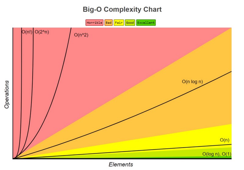
Big O
Go to:
> Material
> Lecture Recap
> Revision Questions
Material
Lecture Recap
Last week we revisited limits and introduced the notion of asymptotic growth, and now you know why! We need them to define the infamous Big-O notation. Only looking at the formulas, the whole thing seems a little whacky at first. We cut factors left and right and somehow everything still behaves the same? Yes but also not quite… Let’s try to get some intuition.
When you implement an algorithm $\mathcal{A}_1(I)$, you’re writing a function that takes in some input instance $I$ and produces an output. On a computer, the input $I$ will be represented as a bit-string of some length $n$. Your computer then processes that bit-string using the set of operations built into its chip—e.g., $+, -, >, \ldots$—each of which takes some number of clock-cycles to execute. How long each of them takes and how they are implemented is determined by the microarchitecture of your computer.1
A Universal Runtime Model
These hardware-specific details make comparing the efficiency of our algorithm by measuring execution time unreliable. Instead, we abstract away from the hardware by creating a universal model. We do this by counting the runtime in terms of the number of basic operations the algorithm carries out. We assume each of these basic operations takes some constant amount of time. While the exact time might differ between machines, this difference is just a constant factor. This allows our analysis to be independent of the specific hardware.
Secondly, we consider its asymptotic behavior—the growth of the runtime as the length of input $I$ approaches $\infty$, i.e., $n \to \infty$. This lets us make general statements about an algorithm’s efficiency that aren’t tied to a specific input size. As you will see in later programming exercises, input lengths can grow very large very quickly, and it’s for these large inputs where runtime really starts to matter.
Caution with Intuition
However, a word of caution for solving exercises: Asymptotics are generally very hard to visually intuit about in specific cases, so don’t let this fool you. For example, an algorithm with a runtime of $1000n$ is asymptotically better than one with a runtime of $n^2$ (i.e., $1000n \in O(n^2)$). However, for any input with size $n < 1000$, the $n^2$ algorithm is actually faster! My advice to you is to stick to the formal definitions and build your intuition that way, rather than trying to plot functions in your head.
Flaws of Big-O
Lastly, while Big-O notation is often a sensible measure, it has its flaws too. Constant factors do count in practice, and the asymptotic view may not always be justified for the problem sizes you’re working with. In later weeks, you will learn about algorithms that look great in Big-O notation on paper but are not feasible to implement in practice because of these hidden constant factors.

Revision Questions
Q1: Why is measuring the runtime of a program in seconds not a reliable or universal way to compare the efficiency of two algorithms?
- Answer: Measuring time in seconds is unreliable because it’s influenced by factors that have nothing to do with the algorithm itself, such as:
- The hardware it’s run on (CPU speed, memory).
- The software environment (operating system, compiler optimizations).
- The goal of algorithm analysis is to find a universal measure that is independent of these factors, which is why we count abstract “basic operations” instead.
Q2: State the formal definition of Big-O. In your own words, what do the constants c and n_0 represent?
- Answer: A function $f(n)$ is in $O(g(n))$ if there exist positive constants
candn_0such that for all $n \ge n_0$, the inequality $0 \le f(n) \le c \cdot g(n)$ holds.crepresents a constant factor. It’s the “headroom” that allows us to ignore less important terms and coefficients.n_0represents a sufficiently large input size. It’s the point from which the asymptotic behavior takes over; we don’t care which function is smaller for inputs less than $n_0$.
Q3: Arrange the following functions in increasing order of asymptotic growth: $f_1(n) = 5n^3 + 100n^2$, $f_2(n) = 1000n^2 \log(n)$, $f_3(n) = 2^n$, and $f_4(n) = 10^8 n^2$.
- Answer: The correct order is $f_4(n) < f_2(n) < f_1(n) < f_3(n)$.
- Both $f_4(n)$ ($O(n^2)$) and $f_1(n)$ ($O(n^3)$) are polynomials. We first compare their degrees.
- $f_2(n)$ ($O(n^2 \log n)$) grows slightly faster than a pure quadratic function ($f_4$) but slower than any cubic function ($f_1$).
- $f_3(n)$ ($O(2^n)$) is an exponential function, which grows asymptotically faster than any polynomial function.
- So, the order is: $O(n^2) < O(n^2 \log n) < O(n^3) < O(2^n)$.
Q4: True or False? $n \log_2(n) \in O(n \log_{10}(n))$. Justify your answer.
- Answer: True.
- Justification: Logarithms with different bases differ only by a constant factor. Using the change of base formula, we can write $\log_2(n) = \frac{\log_{10}(n)}{\log_{10}(2)}$. Since $\frac{1}{\log_{10}(2)}$ is just a constant, the two functions are asymptotically equivalent and the statement holds.
E.g., you might not have elaborate multiplication circuitry but can still implement multiplication using addition — just a tad slower. ↩︎